np.searchsorted is NumPy’s implementation of the binary search algorithm. This is one of the fundamental search algorithms and is used in the Python scientific ecosystem for functionality such as histogram computation and interval lookups. Any optimization benefits libraries such as SciPy and scikit-learn, as well as the broader Python scientific ecosystem.
Several case studies, such as Binary search variants and the effects of batching and Algorithmica’s Binary Search case study explore techniques such as branch elimination, batching, and cache-friendly data layouts to binary search performance. In this post, we explore how those ideas can be expressed using NumPy’s vectorized primitives.
We will derive a vectorized formulation that outperforms NumPy 2.4’s searchsorted implementation, and then port the resulting algorithm back into NumPy. The change was included in NumPy 2.5, achieving up to a 25× speedup in our benchmarks.
searchsorted is also part of the Python Array API Standard. This allows us to compare how different array libraries implement the same operation and exploit parallelism.
Problem definition#
Given a static sorted array and a sequence of query keys, find the insertion position of each key in the array.
A classic pure-Python implementation runs one binary search per key:
def searchsorted_py(a, xs):
    res = np.empty(len(xs), dtype=np.int32)

    for i, x in enumerate(xs):
        lo = 0
        hi = len(a)

        while lo < hi:
            mid = (lo + hi) // 2
            if a[mid] < x:
                lo = mid + 1
            else:
                hi = mid

        res[i] = lo

    return res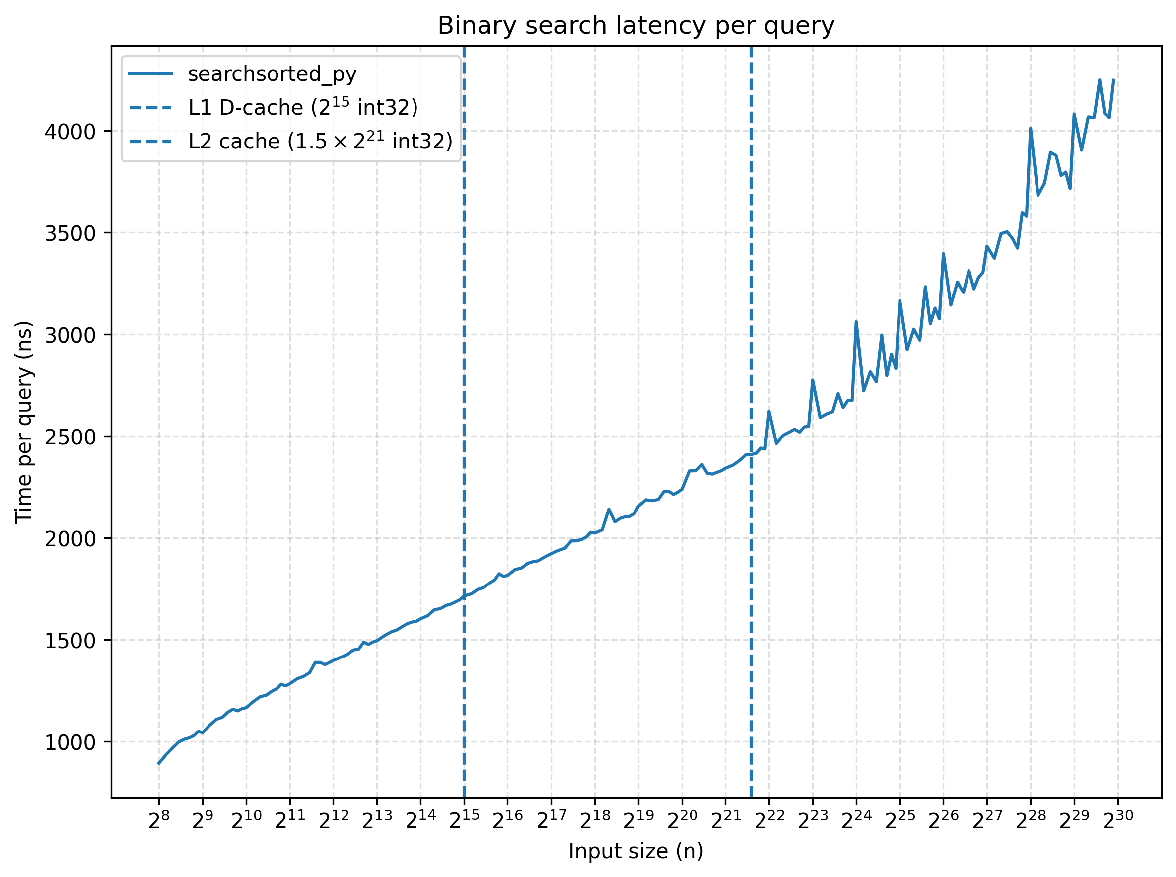
Running time per query grows logarithmically as the input size grows (note the logarithmic scale of x-axis).
For benchmarking, we generated two random arrays of uniformly distributed np.int32 integers. The keys (i.e. the elements being searched) had a fixed length of 10,000, while the length of the sorted array varied up to $2^{30}$ ($4\ GiB$). Both keys and values arrays are contiguous in memory. Each benchmark was repeated 50 times, and we report the minimum execution time.
The benchmarks were run on a MacBook Pro with an Apple M1 Pro and 32 GB of memory. The M1 Pro has 128 KB of L1 data cache per performance core, enough to hold $2^{15}$ 32-bit integers, and a 12 MB L2 cache shared by its performance cores, enough to hold $1.5 * 2^{21}$ 32-bit integers.
Batching with NumPy arrays#
The baseline implementation performs one binary search per query. Each search is independent, but executed sequentially in Python. We can adapt the algorithm so multiple binary searches make progress together in batches. For that we can represent the state of all searches as arrays and update them simultaneously using vectorized operations.
In NumPy, operations on arrays are executed in compiled C++ loops. This removes Python overhead and allows the CPU to efficiently process large batches of independent work.
Let’s vectorize our binary search#
To vectorize the algorithm, we reinterpret scalar variables as array state. Instead of a single lo and hi, we maintain one value per query. In our original implementation, the state consists of lo, hi, and res. Since lo ends up containing the final result, we can focus on tracking just lo and hi.
This first vectorized implementation is a direct translation of the previous algorithm.
def searchsorted_py_np(a, xs):
    lo = np.zeros(xs.shape, dtype=np.int32)
    hi = np.full(xs.shape, len(a), dtype=np.int32)

    while True:
        # True for each element position where lo_i < hi_i
        active = lo < hi
        if not np.any(active):
            # this is basically `while lo < hi:` in the pure-Python version
            break

        mid = (lo + hi) // 2

        # only index those entries where active is true, so we don't modify already computed positions
        mid_a = mid[active]
        xs_a = xs[active]

        mask = a[mid_a] < xs_a

        lo[active] = np.where(mask, mid_a + 1, lo[active])
        hi[active] = np.where(mask, hi[active], mid_a)

    return lo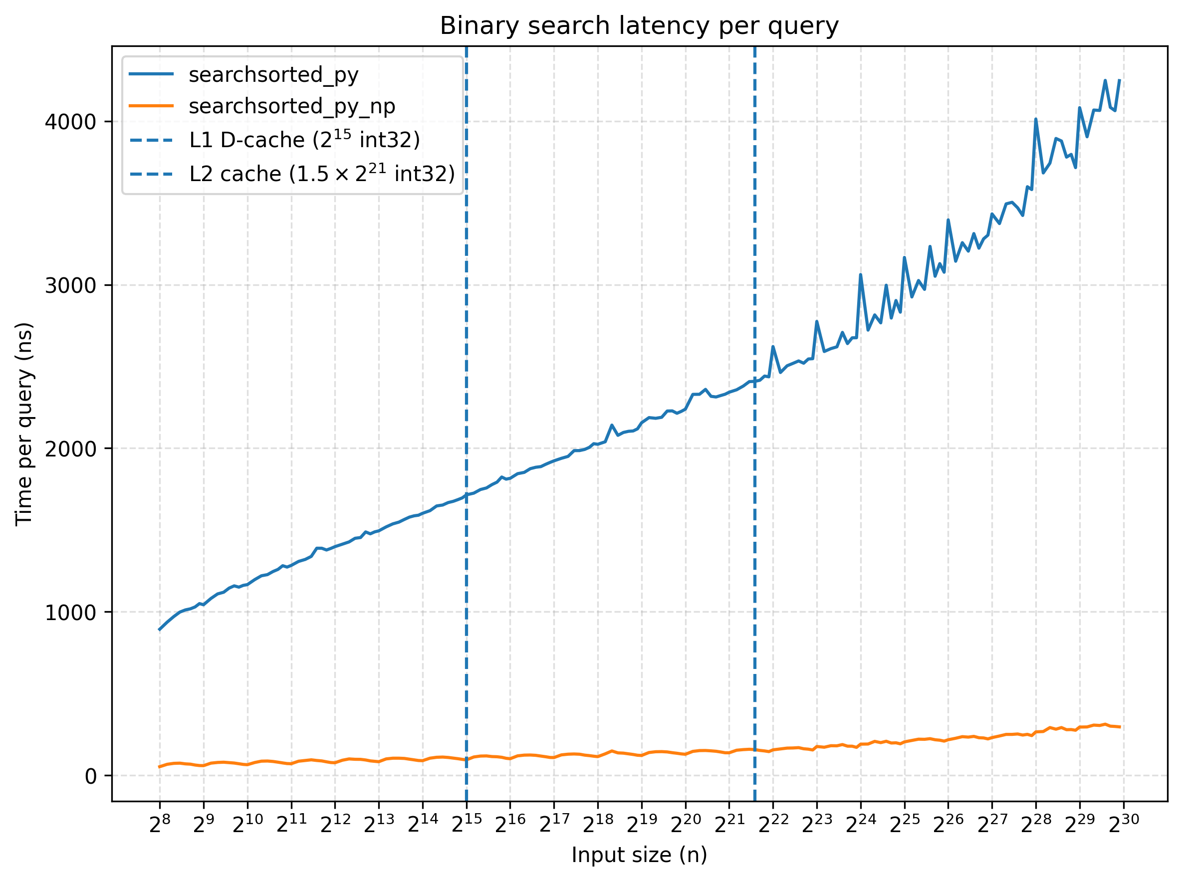
In this implementation, different queries can shrink their search intervals at different rates, so they may require different numbers of iterations to converge.
For example, consider searching for the keys [-1, 2] in the array [0, 1]. For the query 2, the first iteration computes mid = 1 and sets lo = mid + 1 = 2, so the interval becomes [2, 2) and the search converges in one step. For the query -1, the update instead sets hi = mid = 1, leaving the interval [0, 1) after the first step. This requires an additional iteration to collapse the interval to [0, 0).
Because the searches can converge at different times, we need to keep track of which queries are still active. The active mask identifies the queries whose search intervals have not yet converged, allowing us to update only those queries.
Making all searches take the same number of steps#
The important observation is that binary search does not actually need to terminate independently for each key. We can tweak each iteration update in a way that, once a search has converged, subsequent iterations can leave its interval unchanged.
We maintain the invariant that the insertion position lies in [lo, hi). At each iteration, every interval is reduced to roughly half its previous size. After np.ceil(np.log2(n)) iterations, every interval has collapsed to a single position.
For simplicity, this implementation assumes a is non-empty.
def searchsorted_py_np_fixed(a, xs):
    n = len(a)
    lo = np.zeros(xs.shape, dtype=np.int32)
    hi = np.full(xs.shape, n, dtype=np.int32)

    for _ in range(int(np.ceil(np.log2(n)))):
        mid = (lo + hi) // 2
        go_left = xs <= a[mid]

        # for each position i:
        # if go_left_i is True, we keep the `lo_i` value and `hi_i` is updated to `mid_i`
        # if go_left_i is False, we keep the `hi_i` value and `lo_i` is updated to `mid_i`
        lo = np.where(go_left, lo, mid)
        hi = np.where(go_left, mid, hi)

    return hi
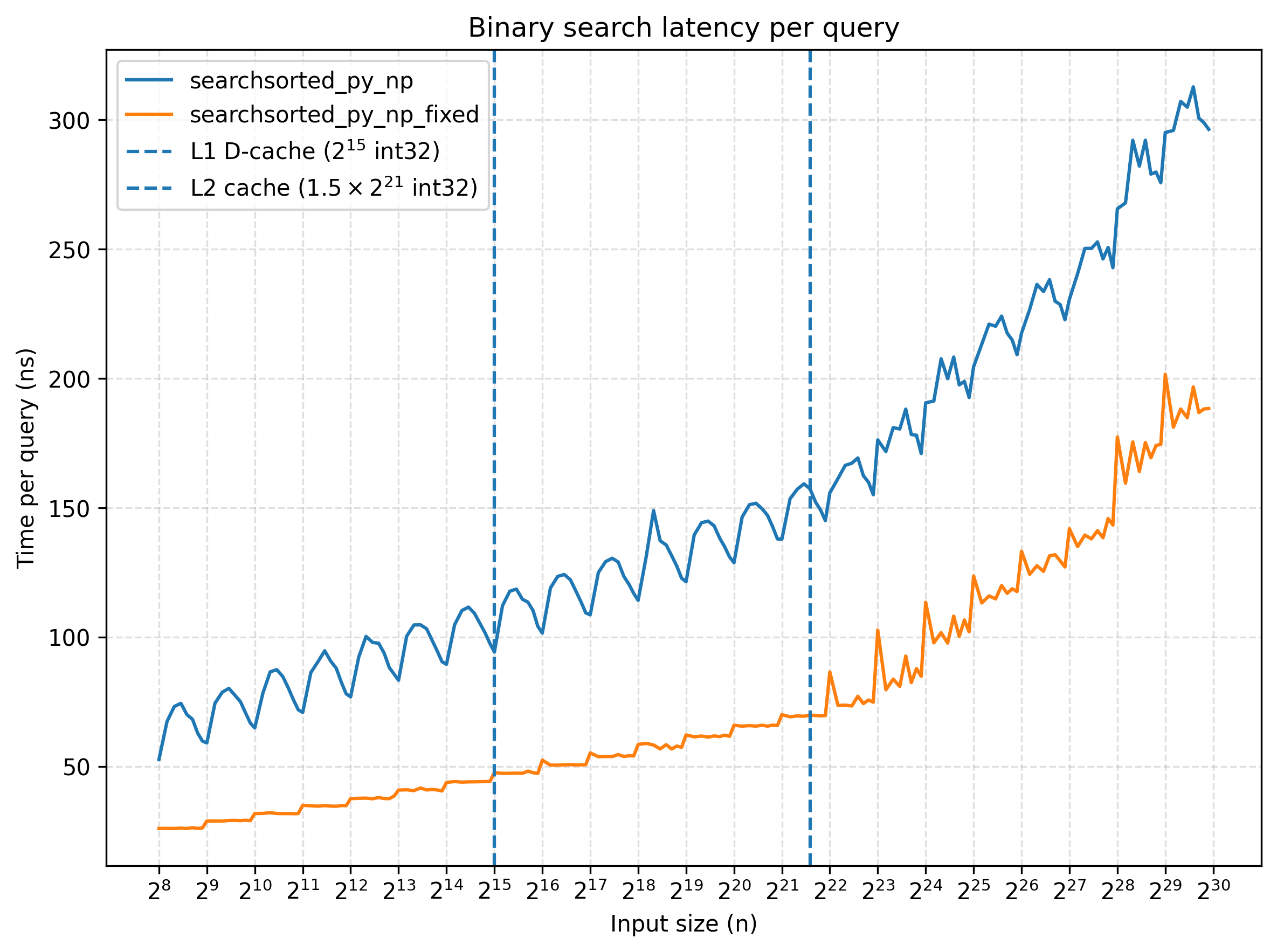
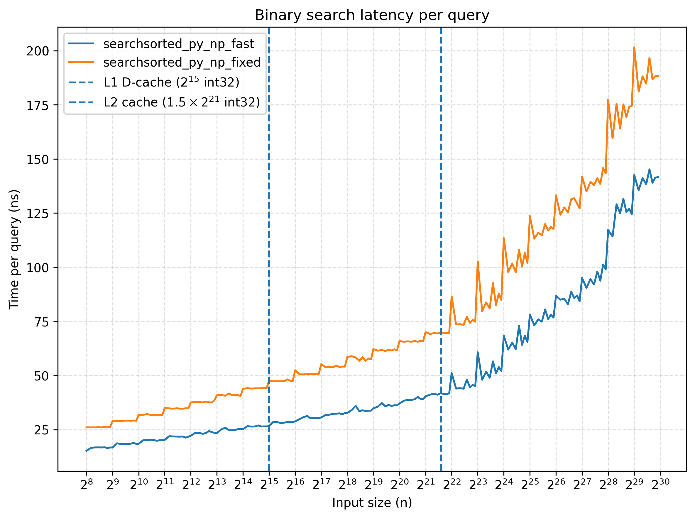
Removing the active tracker makes it up to 2× faster.
A similar formulation can already be found in the Python ecosystem. For example, JAX’s scan-based implementation
...


def body_fun(state, _):
    low, high = state
    mid = low + (high - low) // 2  # use this form to avoid overflow
    go_left = op(query, sorted_arr[mid])
    return (lax.select(go_left, low, mid), lax.select(go_left, mid, high)), ()


n_levels = int(np.ceil(np.log2(n + 1)))
...
Can NumPy beat NumPy?#
Let’s compare the performance of this vectorized implementation with NumPy’s native searchsorted (using NumPy 2.4).
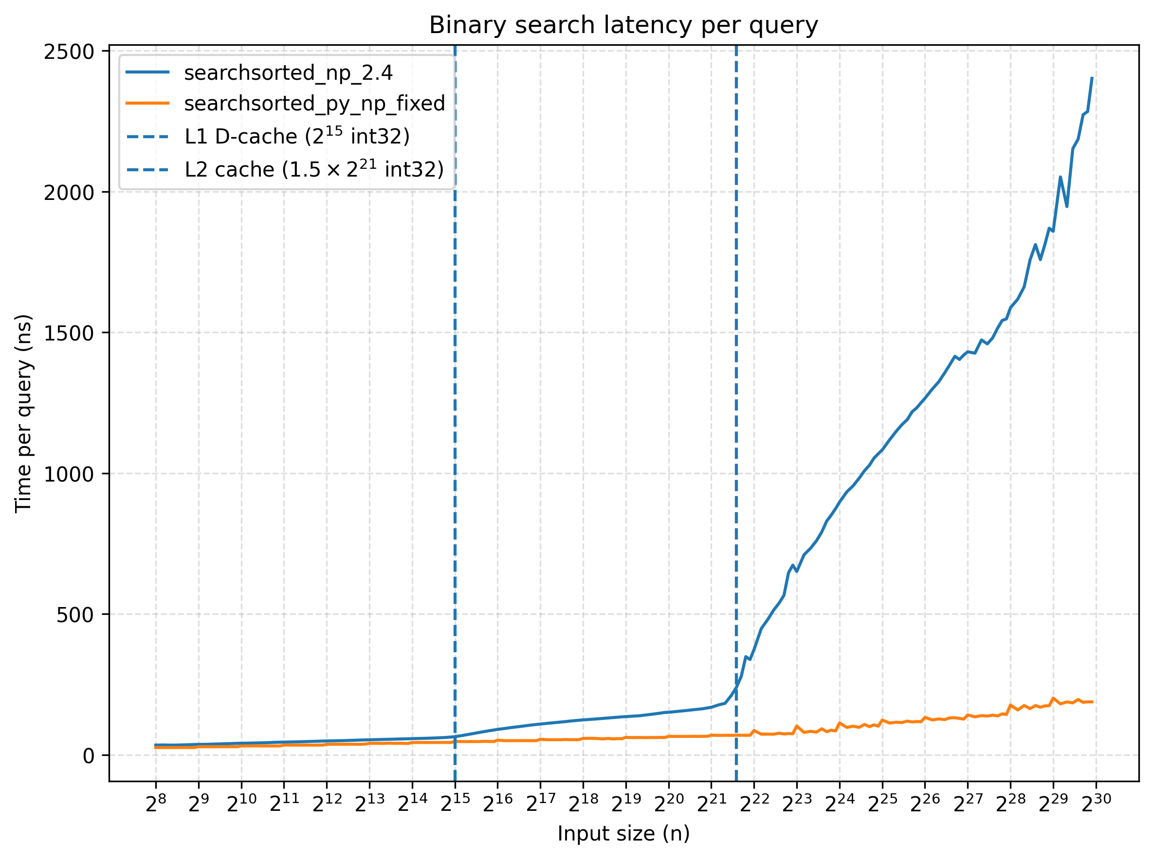
Our vectorized Python implementation can be an order of magnitude faster than the native one for inputs with several keys. To understand why, let’s take a look at NumPy 2.4 implementation:
template <class Tag, side_t side>
static void
binsearch(const char *arr, const char *key, char *ret, npy_intp arr_len,
          npy_intp key_len, npy_intp arr_str, npy_intp key_str,
          npy_intp ret_str, PyArrayObject *)
{
    using T = typename Tag::type;
    auto cmp = side_to_cmp<Tag, side>::value;
    npy_intp min_idx = 0;
    npy_intp max_idx = arr_len;
    T last_key_val;

    if (key_len == 0) {
        return;
    }
    last_key_val = *(const T *)key;

    for (; key_len > 0; key_len--, key += key_str, ret += ret_str) {
        const T key_val = *(const T *)key;
        /*
         * Updating only one of the indices based on the previous key
         * gives the search a big boost when keys are sorted, but slightly
         * slows down things for purely random ones.
         */
        if (cmp(last_key_val, key_val)) {
            max_idx = arr_len;
        }
        else {
            min_idx = 0;
            max_idx = (max_idx < arr_len) ? (max_idx + 1) : arr_len;
        }

        last_key_val = key_val;

        while (min_idx < max_idx) {
            const npy_intp mid_idx = min_idx + ((max_idx - min_idx) >> 1);
            const T mid_val = *(const T *)(arr + mid_idx * arr_str);
            if (cmp(mid_val, key_val)) {
                min_idx = mid_idx + 1;
            }
            else {
                max_idx = mid_idx;
            }
        }
        *(npy_intp *)ret = min_idx;
    }
}
Ignoring the pointer arithmetic details, the core algorithm is a classic binary search executed independently for each key. There is also an optimization that reuses previous search bounds when the input keys are sorted.
This implementation performs one binary search per key, where each search is a fully sequential process. Each iteration of the binary search depends on the result of the previous one (the midpoint determines which part of the array is inspected next). This creates a dependency chain within each search: the next memory access depends on the result of the previous comparison.
For large arrays, binary-search reads also tend to be cache-unfriendly, since each step may require a read from a different cache line. Cache misses have a greater impact on the sequential implementation because each step may stall waiting for the previous memory access to complete.
The vectorized implementation performs the same logical step across all queries at once (all queries advance at each step together). With multiple independent searches, the CPU can have several memory accesses in flight at once. This aligns with the observed running time once the array size exceeds the L1 and L2 cache sizes.
Can we optimize NumPy?#
The previous vectorized implementation maintains two arrays, lo and hi, to represent the search interval for each query. If we were to port this exact implementation into NumPy natively, it would require using $O(K)$ additional memory where K is the number of queries. Even though this approach is potentially faster, this is unacceptable for memory-sensitive workloads.
To reduce the state required, we can reformulate binary search in terms of interval boundaries. Instead of tracking both lo and hi for each query, we describe each interval using its left boundary and its length.
The key observation is that if we structure the algorithm so that all queries shrink their intervals by the same amount at each iteration, then every interval has the same length at each iteration. This means we do not need to store a separate hi per query: it can be reconstructed from a single array lo and a global length. Note that this still needs $O(K)$ space for the output, but it requires only $O(1)$ memory beyond that output.
This gives us the following Python implementation:
def searchsorted_py_np_fast_where(arr, keys):
    K = keys.shape[0]
    length = arr.shape[0]

    base = np.zeros(K, dtype=np.intp)

    # Invariant: the insertion index lies in [base, base + length]
    while length > 1:
        half = length >> 1
        mid = base + half
        base = np.where(keys > arr[mid], mid, base)
        length -= half

    # Final step: result is either base and base + 1
    base = np.where(keys > arr[base], base + 1, base)

    return base
Only a single array base is needed to store the per-query state, while length is shared across all queries. The output is written directly into base, so no additional state array is required. This implementation still requires allocating a temporary mid to hold the midpoints, but this can be avoided in the C++ port.
This formulation is closely related to the branchless binary search approach discussed in Algorithmica’s case study. In the formulation we use, the invariant range is [base, base + length]. Therefore a final step is required when length = 1 to resolve whether the insertion point falls to the left or right of base.
The reformulated implementation is significantly faster:
Porting it into C++#
The performance results show the benefit of reducing the per-query state. We can now translate it almost directly to C++ with $O(1)$ additional memory.
template <class Tag, side_t side>
static void
binsearch(const char *arr, const char *key, char *ret, npy_intp arr_len,
          npy_intp key_len, npy_intp arr_str, npy_intp key_str,
          npy_intp ret_str, PyArrayObject *)
{
    using T = typename Tag::type;
    auto cmp = side_to_cmp<Tag, side>::value;

    // If the array length is 0 we return all 0s
    if (arr_len <= 0) {
        for (npy_intp i = 0; i < key_len; ++i) {
            *(npy_intp *)(ret + i * ret_str) = 0;
        }
        return;
    }

    /*
    base = np.zeros(K, dtype=np.intp)

    We unroll the first iteration for the following reasons:
        1. ret is not initialized with the bases, so we save |keys| writes
        by not having to initialize it with 0s.
        2. By assuming the initial base for every key is 0, we also save
        |keys| reads.
        3. In the first iteration, all elements are compared against the
        median. So we can store it in a variable and use it for all keys.

    This initial block replaces the initialization loop that is used for the
    arr_len==0 case. Note that when arr_len = 1, then half is 0 so the
    following block initializes the array as with 0s.
    */
    npy_intp interval_length = arr_len;
    npy_intp half = interval_length >> 1;
    interval_length -= half; // length -> ceil(length / 2)

    npy_intp base = 0;
    const T mid_val = *(const T *)(arr + (base + half) * arr_str);

    for (npy_intp i = 0; i < key_len; ++i) {
        const T key_val = *(const T *)(key + i * key_str);
        *(npy_intp *)(ret + i * ret_str) = cmp(mid_val, key_val) * half;
    }

    /*
        while length > 1:
            half = length >> 1
            length -= half
            mid = base + half
            base = np.where(keys > arr[mid], mid, base)
    */
    while (interval_length > 1) {
        npy_intp half = interval_length >> 1;
        interval_length -= half;

        for (npy_intp i = 0; i < key_len; ++i) {
            npy_intp &base = *(npy_intp *)(ret + i * ret_str);
            const T mid_val = *(const T *)(arr + (base + half) * arr_str);
            const T key_val = *(const T *)(key + i * key_str);
            base += cmp(mid_val, key_val) * half;
        }
    }

    // base = np.where(keys > arr[base], base + 1, base)
    for (npy_intp i = 0; i < key_len; ++i) {
        npy_intp &base = *(npy_intp *)(ret + i * ret_str);
        const T key_val = *(const T *)(key + i * key_str);
        base += cmp(*(const T *)(arr + base * arr_str), key_val);
    }
}
Note that we exploited a property of the first iteration of the binary search. Because the initial value of every result entry is implicitly zero, we can skip writing and reading those values during the first iteration. Moreover, in the first iteration all elements are compared against the same median, so we can read its value once instead of K times.
This implementation was ported directly into NumPy as part of PR #30517, which was included in the 2.5 release. Now let’s do a final comparison between NumPy 2.4 and 2.5, and our vectorized Python implementation:
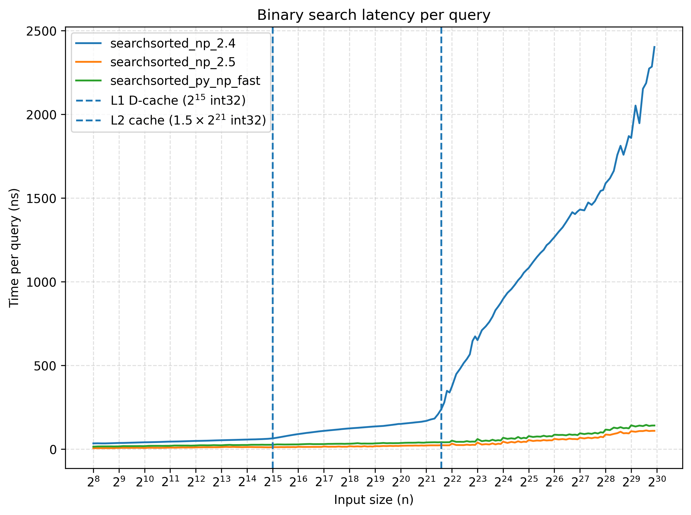
The native 2.5 version is up to 25× faster than NumPy 2.4’s implementation in our benchmarks. Compared with the vectorized Python implementation, the C++ implementation can be up to 2× as fast for smaller arrays. This difference becomes less significant as the array size grows. There is also a memory advantage over the vectorized Python implementation: the Python implementation requires additional arrays to store the search state (low and mid, or base and base + length), whereas the C++ implementation keeps length as a scalar. As a result, the C++ implementation uses only $O(1)$ additional memory, while the NumPy formulation requires memory proportional to the number of queries.
Ecosystem Comparison#
We can compare our optimized NumPy 2.5 against other libraries in the ecosystem. For this experiment, we selected the Python libraries JAX, TensorFlow, and PyTorch.
TensorFlow and PyTorch follow a different approach from JAX and NumPy. While JAX and NumPy leverage vectorized/batched operations to hide memory latency, TensorFlow and PyTorch parallelize independent searches across CPU threads. Search keys are partitioned into batches that are processed by different threads. For more details, see the PyTorch and TensorFlow implementations.
In the benchmarks, we limited parallelism to 8 cores and we increased the number of query keys from 10,000 to 20,000. This gives the multithreaded implementations enough independent work to amortize thread-scheduling overhead.
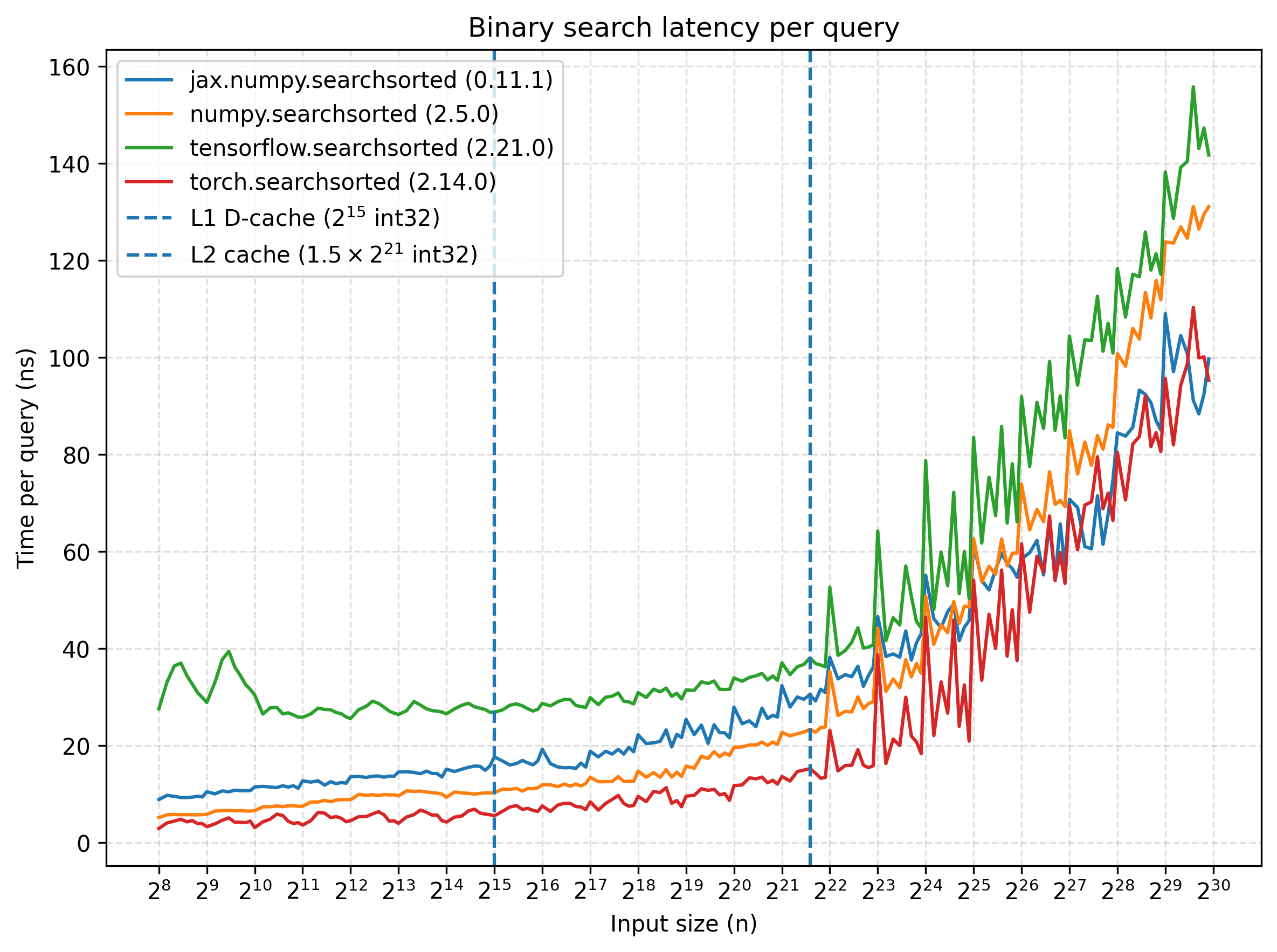
The benchmark shows that NumPy is competitive with the selected libraries in our benchmarks. All implementations exhibit similar behavior once the search array grows beyond the CPU cache.
If we disable multithreading, the performance of PyTorch and TensorFlow degrades, and both exhibit a similar trend to NumPy 2.4’s implementation. Once the search array grows beyond the CPU cache, the cost of memory accesses dominates.
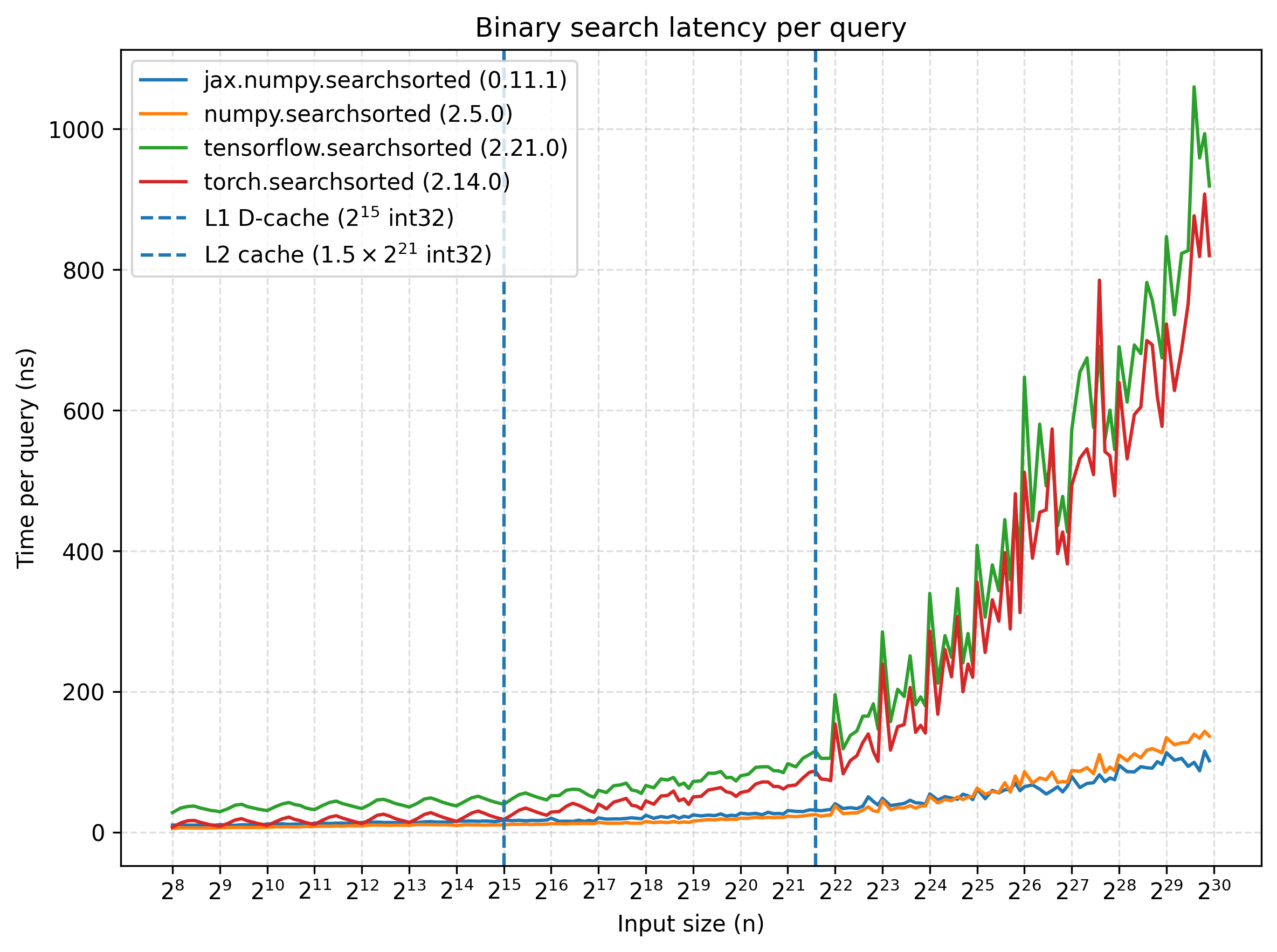
It would be worth benchmarking whether both techniques could be combined: batching binary searches within each thread. However, once the memory subsystem becomes saturated, additional cores can compete for the same memory bandwidth. At that point, improving the memory access patterns may be a more promising direction, for example by using a different layout such as the Eytzinger layout (discussed in detail in the Algorithmica book).
Conclusion#
We made np.searchsorted up to 25x faster in our benchmarks. Given NumPy’s reach in the Python ecosystem, this optimization will benefit several libraries that depend on it. Other libraries in the Python ecosystem with their own binary search implementation may also benefit from adopting similar batching techniques.
Interestingly, we used NumPy array primitives to derive an initial Python implementation that outperformed NumPy 2.4’s implementation. This shows how powerful NumPy’s array primitives can be for implementing highly performant algorithms. A vectorized NumPy implementation in Python can outperform a scalar native implementation by exploiting independent work.
Cache-friendly layouts such as the Eytzinger layout are another interesting direction for making searchsorted faster. It would be interesting to explore whether the array API could expose such layouts through an interface like searchsorted(arr, keys, layout="eytzinger"), although this would require carefully defining the API semantics since the Eytzinger representation is not sorted.