As part of the University of North Carolina BIOL222 class, Dr. Catherine Kehl asked her students to “use matplotlib.pyplot to make art.” BIOL222 is Introduction to Programming, aimed at students with no programming background. The emphasis is on practical, hands-on active learning.
The students completed the assignment with festive enthusiasm around Halloween. Here are some great examples:
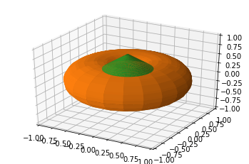
Harris Davis showed an affinity for pumpkins, opting to go 3D!
# get library for 3d plotting
from mpl_toolkits.mplot3d import Axes3D
# make a pumpkin :)
rho = np.linspace(0, 3 * np.pi, 32)
theta, phi = np.meshgrid(rho, rho)
r, R = 0.5, 0.5
X = (R + r * np.cos(phi)) * np.cos(theta)
Y = (R + r * np.cos(phi)) * np.sin(theta)
Z = r * np.sin(phi)
# make the stem
theta1 = np.linspace(0, 2 * np.pi, 90)
r1 = np.linspace(0, 3, 50)
T1, R1 = np.meshgrid(theta1, r1)
X1 = R1 * 0.5 * np.sin(T1)
Y1 = R1 * 0.5 * np.cos(T1)
Z1 = -(np.sqrt(X1**2 + Y1**2) - 0.7)
Z1[Z1 < 0.3] = np.nan
Z1[Z1 > 0.7] = np.nan
# Display the pumpkin & stem
fig = plt.figure()
ax = fig.gca(projection="3d")
ax.set_xlim3d(-1, 1)
ax.set_ylim3d(-1, 1)
ax.set_zlim3d(-1, 1)
ax.plot_surface(X, Y, Z, color="tab:orange", rstride=1, cstride=1)
ax.plot_surface(X1, Y1, Z1, color="tab:green", rstride=1, cstride=1)
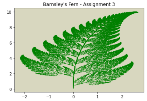
plt.show()Bryce Desantis stuck to the biological theme and demonstrated fractal art.
import numpy as np
import matplotlib.pyplot as plt

# Barnsley's Fern - Fractal; en.wikipedia.org/wiki/Barnsley_…


# functions for each part of fern:
# stem
def stem(x, y):
    return (0, 0.16 * y)


# smaller leaflets
def smallLeaf(x, y):
    return (0.85 * x + 0.04 * y, -0.04 * x + 0.85 * y + 1.6)


# large left leaflets
def leftLarge(x, y):
    return (0.2 * x - 0.26 * y, 0.23 * x + 0.22 * y + 1.6)


# large right leftlets
def rightLarge(x, y):
    return (-0.15 * x + 0.28 * y, 0.26 * x + 0.24 * y + 0.44)


componentFunctions = [stem, smallLeaf, leftLarge, rightLarge]

# number of data points and frequencies for parts of fern generated:
# lists with all 75000 datapoints
datapoints = 75000
x, y = 0, 0
datapointsX = []
datapointsY = []
# For 75,000 datapoints
for n in range(datapoints):
    FrequencyFunction = np.random.choice(componentFunctions, p=[0.01, 0.85, 0.07, 0.07])
    x, y = FrequencyFunction(x, y)
    datapointsX.append(x)
    datapointsY.append(y)

# Scatter plot & scaled down to 0.1 to show more definition:
plt.scatter(datapointsX, datapointsY, s=0.1, color="g")
# Title of Figure
plt.title("Barnsley's Fern - Assignment 3")
# Changing background color
ax = plt.axes()
ax.set_facecolor("#d8d7bf")
Grace Bell got a little trippy with this rotationally semetric art. It’s pretty cool how she captured mouse events. It reminds us of a flower. What do you see?
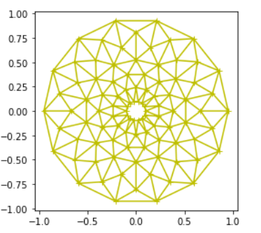
import matplotlib.pyplot as plt
from matplotlib.tri import Triangulation
from matplotlib.patches import Polygon
import numpy as np
# I found this sample code online and manipulated it to make the art piece!
# was interested in because it combined what we used for functions as well as what we used for plotting with (x,y)
def update_polygon(tri):
if tri == -1:
points = [0, 0, 0]
else:
points = triang.triangles[tri]
xs = triang.x[points]
ys = triang.y[points]
polygon.set_xy(np.column_stack([xs, ys]))
def on_mouse_move(event):
if event.inaxes is None:
tri = -1
else:
tri = trifinder(event.xdata, event.ydata)
update_polygon(tri)
ax.set_title(f"In triangle {tri}")
event.canvas.draw()
# this is the info that creates the angles
n_angles = 14
n_radii = 7
min_radius = 0.1 # the radius of the middle circle can move with this variable
radii = np.linspace(min_radius, 0.95, n_radii)
angles = np.linspace(0, 2 * np.pi, n_angles, endpoint=False)
angles = np.repeat(angles[..., np.newaxis], n_radii, axis=1)
angles[:, 1::2] += np.pi / n_angles
x = (radii * np.cos(angles)).flatten()
y = (radii * np.sin(angles)).flatten()
triang = Triangulation(x, y)
triang.set_mask(
np.hypot(x[triang.triangles].mean(axis=1), y[triang.triangles].mean(axis=1))
< min_radius
)
trifinder = triang.get_trifinder()
fig, ax = plt.subplots(subplot_kw={"aspect": "equal"})
ax.triplot(
triang, "y+-"
) # made the color of the plot yellow and there are "+" for the data points but you can't really see them because of the lines crossing
polygon = Polygon([[0, 0], [0, 0]], facecolor="y")
update_polygon(-1)
ax.add_patch(polygon)
fig.canvas.mpl_connect("motion_notify_event", on_mouse_move)
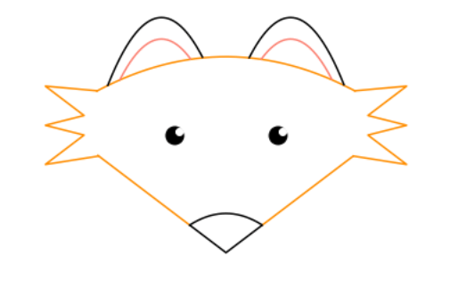
plt.show()As a bonus, did you like that fox in the banner? That was created (and well documented) by Emily Foster!
import numpy as np
import matplotlib.pyplot as plt

plt.axis("off")

# head
xhead = np.arange(-50, 50, 0.1)
yhead = -0.007 * (xhead * xhead) + 100

plt.plot(xhead, yhead, "darkorange")

# outer ears
xearL = np.arange(-45.8, -9, 0.1)
yearL = -0.08 * (xearL * xearL) - 4 * xearL + 70

xearR = np.arange(9, 45.8, 0.1)
yearR = -0.08 * (xearR * xearR) + 4 * xearR + 70

plt.plot(xearL, yearL, "black")
plt.plot(xearR, yearR, "black")

# inner ears
xinL = np.arange(-41.1, -13.7, 0.1)
yinL = -0.08 * (xinL * xinL) - 4 * xinL + 59

xinR = np.arange(13.7, 41.1, 0.1)
yinR = -0.08 * (xinR * xinR) + 4 * xinR + 59

plt.plot(xinL, yinL, "salmon")
plt.plot(xinR, yinR, "salmon")

# bottom of face
xfaceL = np.arange(-49.6, -14, 0.1)
xfaceR = np.arange(14, 49.3, 0.1)
xfaceM = np.arange(-14, 14, 0.1)

plt.plot(xfaceL, abs(xfaceL), "darkorange")
plt.plot(xfaceR, abs(xfaceR), "darkorange")
plt.plot(xfaceM, abs(xfaceM), "black")

# nose
xnose = np.arange(-14, 14, 0.1)
ynose = -0.03 * (xnose * xnose) + 20

plt.plot(xnose, ynose, "black")

# whiskers
xwhiskR = [50, 70, 55, 70, 55, 70, 49.3]
xwhiskL = [-50, -70, -55, -70, -55, -70, -49.3]
ywhisk = [82.6, 85, 70, 65, 60, 45, 49.3]

plt.plot(xwhiskR, ywhisk, "darkorange")
plt.plot(xwhiskL, ywhisk, "darkorange")

# eyes
plt.plot(20, 60, color="black", marker="o", markersize=15)
plt.plot(-20, 60, color="black", marker="o", markersize=15)

plt.plot(22, 62, color="white", marker="o", markersize=6)
plt.plot(-18, 62, color="white", marker="o", markersize=6)
We look forward to seeing these students continue in their plotting and scientific adventures!