In May 2020, Alexandre Morin-Chassé published a blog post about the stellar chart. This type of chart is an (approximately) direct alternative to the radar chart (also known as web, spider, star, or cobweb chart) — you can read more about this chart here.
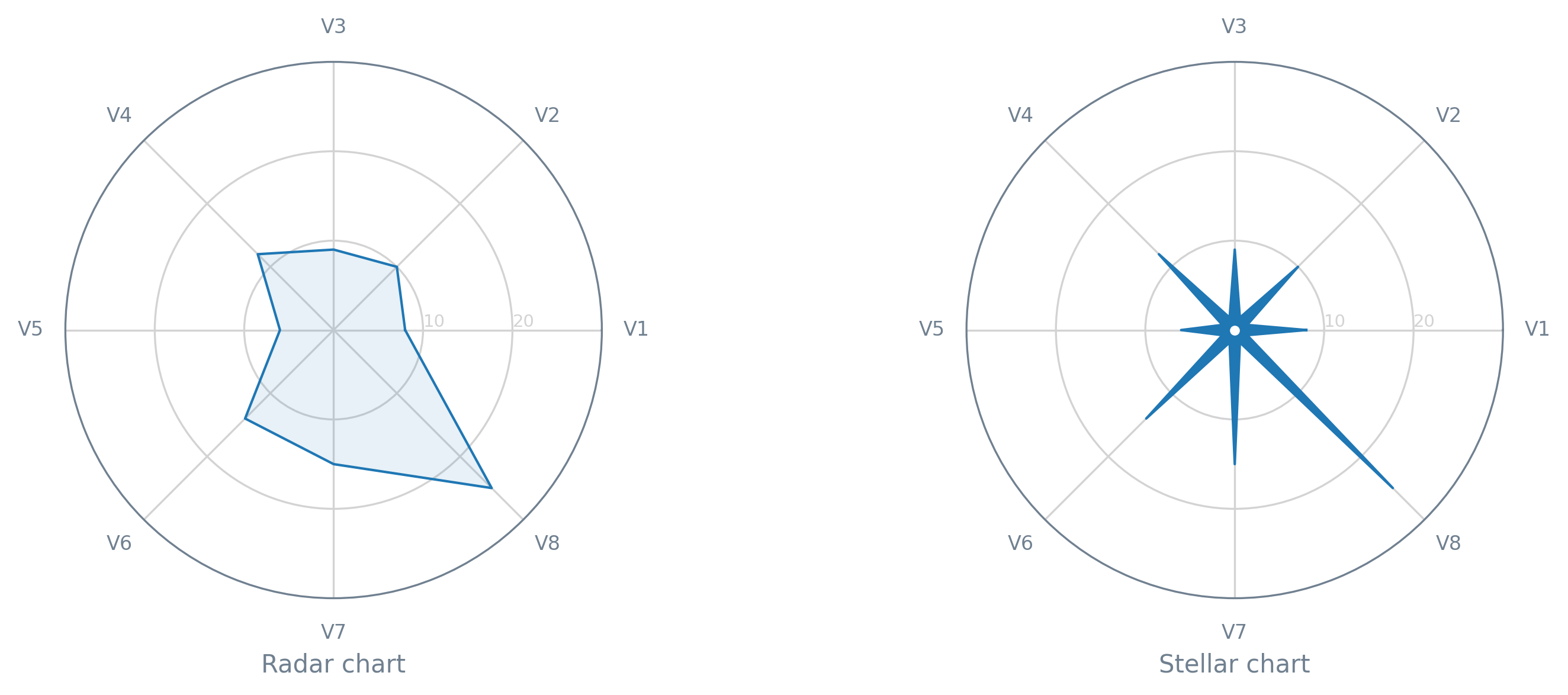
In this tutorial, we will see how we can create a quick-and-dirty stellar chart. First of all, let’s get the necessary modules/libraries, as well as prepare a dummy dataset (with just a single record).
from itertools import chain, zip_longest
from math import ceil, pi

import matplotlib.pyplot as plt

data = [
    ("V1", 8),
    ("V2", 10),
    ("V3", 9),
    ("V4", 12),
    ("V5", 6),
    ("V6", 14),
    ("V7", 15),
    ("V8", 25),
]
We will also need some helper functions, namely a function to round up to the nearest 10 (round_up()) and a function to join two sequences (even_odd_merge()). In the latter, the values of the first sequence (a list or a tuple, basically) will fill the even positions and the values of the second the odd ones.
def round_up(value):
    """
    >>> round_up(25)
    30
    """
    return int(ceil(value / 10.0)) * 10


def even_odd_merge(even, odd, filter_none=True):
    """
    >>> list(even_odd_merge([1,3], [2,4]))
    [1, 2, 3, 4]
    """
    if filter_none:
        return filter(None.__ne__, chain.from_iterable(zip_longest(even, odd)))

    return chain.from_iterable(zip_longest(even, odd))
That said, to plot data on a stellar chart, we need to apply some transformations, as well as calculate some auxiliary values. So, let’s start by creating a function (prepare_angles()) to calculate the angle of each axis on the chart (N corresponds to the number of variables to be plotted).
def prepare_angles(N):
    angles = [n / N * 2 * pi for n in range(N)]

    # Repeat the first angle to close the circle
    angles += angles[:1]

    return angles
Next, we need a function (prepare_data()) responsible for adjusting the original data (data) and separating it into several easy-to-use objects.
def prepare_data(data):
    labels = [d[0] for d in data]  # Variable names
    values = [d[1] for d in data]

    # Repeat the first value to close the circle
    values += values[:1]

    N = len(labels)
    angles = prepare_angles(N)

    return labels, values, angles, N
Lastly, for this specific type of chart, we require a function (prepare_stellar_aux_data()) that, from the previously calculated angles, prepares two lists of auxiliary values: a list of intermediate angles for each pair of angles (stellar_angles) and a list of small constant values (stellar_values), which will act as the values of the variables to be plotted in order to achieve the star-like shape intended for the stellar chart.
def prepare_stellar_aux_data(angles, ymax, N):
    angle_midpoint = pi / N

    stellar_angles = [angle + angle_midpoint for angle in angles[:-1]]
    stellar_values = [0.05 * ymax] * N

    return stellar_angles, stellar_values
At this point, we already have all the necessary ingredients for the stellar chart, so let’s move on to the Matplotlib side of this tutorial. In terms of aesthetics, we can rely on a function (draw_peripherals()) designed for this specific purpose (feel free to customize it!).
def draw_peripherals(ax, labels, angles, ymax, outer_color, inner_color):
    # X-axis
    ax.set_xticks(angles[:-1])
    ax.set_xticklabels(labels, color=outer_color, size=8)

    # Y-axis
    ax.set_yticks(range(10, ymax, 10))
    ax.set_yticklabels(range(10, ymax, 10), color=inner_color, size=7)
    ax.set_ylim(0, ymax)
    ax.set_rlabel_position(0)

    # Both axes
    ax.set_axisbelow(True)

    # Boundary line
    ax.spines["polar"].set_color(outer_color)

    # Grid lines
    ax.xaxis.grid(True, color=inner_color, linestyle="-")
    ax.yaxis.grid(True, color=inner_color, linestyle="-")
To plot the data and orchestrate (almost) all the steps necessary to have a stellar chart, we just need one last function: draw_stellar().
def draw_stellar(
    ax,
    labels,
    values,
    angles,
    N,
    shape_color="tab:blue",
    outer_color="slategrey",
    inner_color="lightgrey",
):
    # Limit the Y-axis according to the data to be plotted
    ymax = round_up(max(values))

    # Get the lists of angles and variable values
    # with the necessary auxiliary values injected
    stellar_angles, stellar_values = prepare_stellar_aux_data(angles, ymax, N)
    all_angles = list(even_odd_merge(angles, stellar_angles))
    all_values = list(even_odd_merge(values, stellar_values))

    # Apply the desired style to the figure elements
    draw_peripherals(ax, labels, angles, ymax, outer_color, inner_color)

    # Draw (and fill) the star-shaped outer line/area
    ax.plot(
        all_angles,
        all_values,
        linewidth=1,
        linestyle="solid",
        solid_joinstyle="round",
        color=shape_color,
    )

    ax.fill(all_angles, all_values, shape_color)

    # Add a small hole in the center of the chart
    ax.plot(0, 0, marker="o", color="white", markersize=3)
Finally, let’s get our chart on a blank canvas (figure).
fig = plt.figure(dpi=100)
ax = fig.add_subplot(111, polar=True)  # Don't forget the projection!

draw_stellar(ax, *prepare_data(data))

plt.show()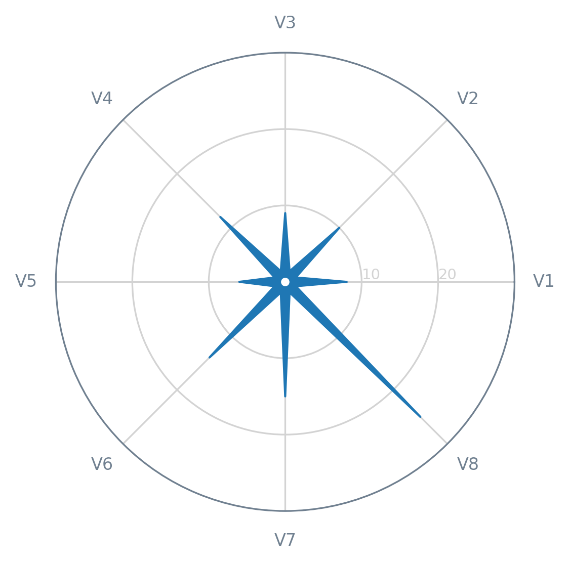
It’s done! Right now, you have an example of a stellar chart and the boilerplate code to add this type of chart to your repertoire. If you end up creating your own stellar charts, feel free to share them with the world (and me!). I hope this tutorial was useful and interesting for you!