The last and final post discussing the VF2++ helpers can be found here. Now that we’ve figured out how to solve all the sub-problems that VF2++ consists of, we are ready to combine our implemented functionalities to create the final solver for the Graph Isomorphism problem.
Introduction#
We should quickly review the individual functionalities used in the VF2++ algorithm:
- Node ordering which finds the optimal order to access the nodes, such that those that are more likely to match are placed first in the order. This reduces the possibility of infeasible searches taking place first.
- Candidate selection such that, given a node $u$ from $G_1$, we obtain the candidate nodes $v$ from $G_2$.
- Feasibility rules introducing easy-to-check cutting and consistency conditions which, if satisfied by a candidate pair of nodes $u$ from $G_1$ and $v$ from $G_2$, the mapping is extended.
- $T_i$ updating which updates the $T_i$ and $\tilde{T}_i$, $i=1,2$ parameters in case that a new pair is added to the mapping, and restores them when a pair is popped from it.
We are going to use all these functionalities to form our Isomorphism solver.
VF2++#
First of all, let’s describe the algorithm in simple terms, before presenting the pseudocode. The algorithm will look something like this:
- Check if all preconditions are satisfied before calling the actual solver. For example there’s no point examining two graphs with different number of nodes for isomorphism.
- Initialize all the necessary parameters ($T_i$, $\tilde{T}_i$, $i=1,2$) and maybe cache some information that is going to be used later.
- Take the next unexamined node $u$ from the ordering.
- Find its candidates and check if there’s a candidate $v$ such that the pair $u-v$ satisfies the feasibility rules
- if there’s any, extend the mapping and go to 3.
- if not, pop the last pair $\hat{u}-\hat{v}$ from the mapping and try a different candidate $\hat{v}$, from the remaining candidates of $\hat{u}$
- The two graphs are isomorphic if the number of mapped nodes equals the number of nodes of the two graphs.
- The two graphs are not isomorphic if there are no remaining candidates for the first node of the ordering (root).
The official code for the VF2++ is presented below.
# Check if there's a graph with no nodes in it
if G1.number_of_nodes() == 0 or G2.number_of_nodes() == 0:
    return False

# Check that both graphs have the same number of nodes and degree sequence
if not nx.faster_could_be_isomorphic(G1, G2):
    return False

# Initialize parameters (Ti/Ti_tilde, i=1,2) and cache necessary information about degree and labels
graph_params, state_params = _initialize_parameters(G1, G2, node_labels, default_label)

# Check if G1 and G2 have the same labels, and that number of nodes per label is equal between the two graphs
if not _precheck_label_properties(graph_params):
    return False

# Calculate the optimal node ordering
node_order = _matching_order(graph_params)

# Initialize the stack to contain node-candidates pairs
stack = []
candidates = iter(_find_candidates(node_order[0], graph_params, state_params))
stack.append((node_order[0], candidates))

mapping = state_params.mapping
reverse_mapping = state_params.reverse_mapping

# Index of the node from the order, currently being examined
matching_node = 1

while stack:
    current_node, candidate_nodes = stack[-1]

    try:
        candidate = next(candidate_nodes)
    except StopIteration:
        # If no remaining candidates, return to a previous state, and follow another branch
        stack.pop()
        matching_node -= 1
        if stack:
            # Pop the previously added u-v pair, and look for a different candidate _v for u
            popped_node1, _ = stack[-1]
            popped_node2 = mapping[popped_node1]
            mapping.pop(popped_node1)
            reverse_mapping.pop(popped_node2)
            _restore_Tinout(popped_node1, popped_node2, graph_params, state_params)
        continue

    if _feasibility(current_node, candidate, graph_params, state_params):
        # Terminate if mapping is extended to its full
        if len(mapping) == G2.number_of_nodes() - 1:
            cp_mapping = mapping.copy()
            cp_mapping[current_node] = candidate
            yield cp_mapping
            continue

        # Feasibility rules pass, so extend the mapping and update the parameters
        mapping[current_node] = candidate
        reverse_mapping[candidate] = current_node
        _update_Tinout(current_node, candidate, graph_params, state_params)
        # Append the next node and its candidates to the stack
        candidates = iter(
            _find_candidates(node_order[matching_node], graph_params, state_params)
        )
        stack.append((node_order[matching_node], candidates))
matching_node += 1Performance#
This section is dedicated to the performance comparison between VF2 and VF2++. The comparison was performed in random graphs without labels, for number of nodes anywhere between the range $(100-2000)$. The results are depicted in the two following diagrams.
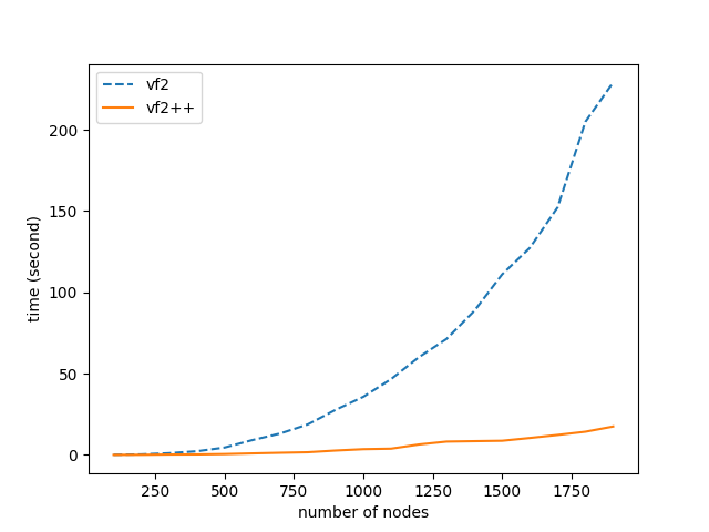
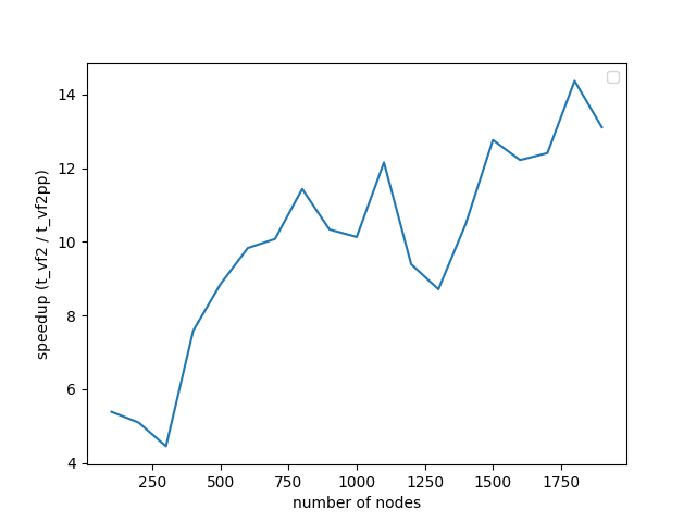
We notice that the maximum speedup achieved is 14x, and continues to increase as the number of nodes increase. It is also highly prominent that the increase in number of nodes, doesn’t seem to affect the performance of VF2++ to a significant extent, when compared to the drastic impact on the performance of VF2. Our results are almost identical to those presented in the original VF2++ paper, verifying the theoretical analysis and premises of the literature.
Optimizations#
The achieved boost is due to some key improvements and optimizations, specifically:
- Optimal node ordering, which avoids following unfruitful branches that will result in infeasible states. We make sure that the nodes that have the biggest possibility to match are accessed first.
- Implementation in a non-recursive manner, avoiding Python’s maximum recursion limit while also reducing function call overhead.
- Caching of both node degrees and nodes per degree in the beginning, so that we don’t have to access those features in every degree check. For example, instead of doing
res = []
for node in G2.nodes():
    if G1.degree[u] == G2.degree[node]:
        res.append(node)
# do stuff with res ...
to get the nodes of same degree as u (which happens a lot of times in the implementation), we just do:
res = G2_nodes_of_degree[G1.degree[u]]
# do stuff with res ...
where “G2_nodes_of_degree” stores set of nodes for a given degree. The same is done with node labels.
- Extra shrinking of the candidate set for each node by adding more checks in the candidate selection method and removing some from the feasibility checks. In simple terms, instead of checking a lot of conditions on a larger set of candidates, we check fewer conditions but on a more targeted and significantly smaller set of candidates. For example, in this code:
candidates = set(G2.nodes())
for candidate in candidates:
    if feasibility(u, candidate):
        do_stuff()
we take a huge set of candidates, which results in poor performance due to maximizing calls of “feasibility”, thus performing the feasibility checks in a very large set. Now compare that to the following alternative:
candidates = [
    n
    for n in G2_nodes_of_degree[G1.degree[u]].intersection(
        G2_nodes_of_label[G1_labels[u]]
    )
]
for candidate in candidates:
    if feasibility(u, candidate):
        do_stuff()
Immediately we have drastically reduced the number of checks performed and calls to the function, as now we only apply them to nodes of the same degree and label as $u$. This is a simplification for demonstration purposes. In the actual implementation there are more checks and extra shrinking of the candidate set.
Demo#
Let’s demonstrate our VF2++ solver on a real graph. We are going to use the graph from the Graph Isomorphism wikipedia.


Let’s start by constructing the graphs from the image above. We’ll call
the graph on the left G and the graph on the left H:
import networkx as nx

G = nx.Graph(
    [
        ("a", "g"),
        ("a", "h"),
        ("a", "i"),
        ("g", "b"),
        ("g", "c"),
        ("b", "h"),
        ("b", "j"),
        ("h", "d"),
        ("c", "i"),
        ("c", "j"),
        ("i", "d"),
        ("d", "j"),
    ]
)

H = nx.Graph(
    [
        (1, 2),
        (1, 5),
        (1, 4),
        (2, 6),
        (2, 3),
        (3, 7),
        (3, 4),
        (4, 8),
        (5, 6),
        (5, 8),
        (6, 7),
        (7, 8),
    ]
)
use the VF2++ without taking labels into consideration#
res = nx.vf2pp_is_isomorphic(G, H, node_label=None)
# res: True

res = nx.vf2pp_isomorphism(G, H, node_label=None)
# res: {1: "a", 2: "h", 3: "d", 4: "i", 5: "g", 6: "b", 7: "j", 8: "c"}

res = list(nx.vf2pp_all_isomorphisms(G, H, node_label=None))
# res: all isomorphic mappings (there might be more than one). This function is a generator.
use the VF2++ taking labels into consideration#
# Assign some label to each node
G_node_attributes = {
    "a": "blue",
    "g": "green",
    "b": "pink",
    "h": "red",
    "c": "yellow",
    "i": "orange",
    "d": "cyan",
    "j": "purple",
}

nx.set_node_attributes(G, G_node_attributes, name="color")

H_node_attributes = {
    1: "blue",
    2: "red",
    3: "cyan",
    4: "orange",
    5: "green",
    6: "pink",
    7: "purple",
    8: "yellow",
}

nx.set_node_attributes(H, H_node_attributes, name="color")

res = nx.vf2pp_is_isomorphic(G, H, node_label="color")
# res: True

res = nx.vf2pp_isomorphism(G, H, node_label="color")
# res: {1: "a", 2: "h", 3: "d", 4: "i", 5: "g", 6: "b", 7: "j", 8: "c"}

res = list(nx.vf2pp_all_isomorphisms(G, H, node_label="color"))
# res: {1: "a", 2: "h", 3: "d", 4: "i", 5: "g", 6: "b", 7: "j", 8: "c"}
Notice how in the first case, our solver may return a different mapping every time, since the absence of labels results in nodes that can map to more than one others. For example, node 1 can map to both a and h, since the graph is symmetrical.
On the second case though, the existence of a single, unique label per node imposes that there’s only one match for each node, so the mapping returned is deterministic. This is easily observed from
output of list(nx.vf2pp_all_isomorphisms) which, in the first case, returns all possible mappings while in the latter, returns a single, unique isomorphic mapping.