
My implementation of asadpour_atsp is now working!
Recall that my pseudo code for this function from my last post was
def asadpour_tsp
    Input: A complete graph G with weight being the attribute key for the edge weights.
    Output: A list of edges which form the approximate ATSP solution.

    z_star = held_karp(G)
    # test to see if z_star is a graph or dict
    if type(z_star) is nx.DiGraph
        return z_star.edges

    z_support = nx.MultiGraph()
    for u, v in z_star
        if not in z_support.edges
            edge_weight = min(G[u][v][weight], G[v][u][weight])
            z_support.add_edge(u, v, weight=edge_weight)
    gamma = spanning_tree_distribution(z_support, z_star)

    for u, v in z_support.edges
        z_support[u][v][lambda] = exp(gamma[(u, v)])

    for _ in range 1 to 2 ceil(log(n))
        sampled_tree = sample_spanning_tree(G)
        sampled_tree_weight = sampled_tree.size()
        if sampled_tree_weight < minimum_sampled_tree_weight
            minimum_sampled_tree = sampled_tree.copy()
            minimum_sampled_tree_weight = sampled_tree_weight

    t_star = nx.DiGraph
    for u, v, d in minimum_sampled_tree.edges(data=weight)
        if d == G[u][v][weight]
            t_star.add_edge(u, v, weight=d)
        else
            t_star.add_edge(v, u, weight=d)

    for n in t_star
        node_demands[n] = t_star.out_degree(n) - t_star.in_degree(n)

    nx.set_node_attributes(G, node_demands)
    flow_dict = nx.min_cost_flow(G)

     for u, v in flow_dict
        if edge not in t_star.edges and flow_dict[u, v] > 0
            t_star.add_edge(u, v)
    eulerian_curcuit = nx.eulerian_circuit(t_star)
    return _shortcutting(eulerian_curcuit)
And this was more or less correct. A few issues were present, as they always were going to be.
First, my largest issue came from a part of a word being in parenthesis in the Asadpour paper on page 385.
This integral circulation $f^*$ corresponds to a directed (multi)graph $H$ which contains $\vec{T}^*$.
Basically if the minimum flow is every larger than 1 along an edge, I need to add that many parallel edges in order to ensure that everything is still Eulerian. This became a problem quickly while developing my test cases as shown in the below example.
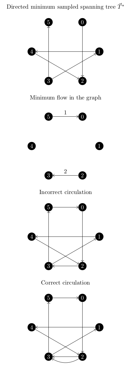
As you can see, for the incorrect circulation, vertices 2 and 3 are not eulerian as they in and out degrees do not match.
All of the others were just minor points where the pseudo code didn’t directly translate into python (because, after all, it isn’t python).
Understanding the Output#
The first thing I did once asadpour_atsp was take the fractional, symmetric Held Karp relaxation test graph and run it through the general traveling_salesman_problem function.
Since there are random numbers involved here, the results were always within the $O(\log n / \log \log n)$ approximation factor but were different.
Three examples are shown below.
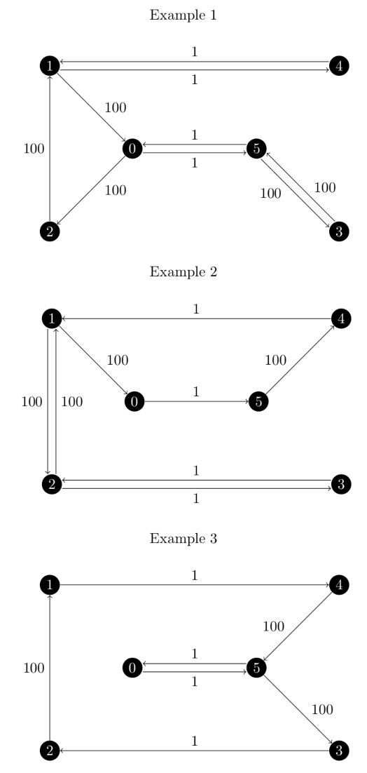
The first thing we want to check is the approximation ratio.
We know that the minimum cost output of the traveling_saleman_problem function is 304 (This is actually lower than the optimal tour in the undirected version, more on this later).
Next we need to know what our maximum approximation factor is.
Now, the Asadpour algorithm is $O(\log n / \log \log n)$ which for our six vertex graph would be $\ln(6) / \ln(\ln(6)) \approx 3.0723$.
However, on page 386 they give the coefficients of the approximation as $(2 + 8 \log n / \log \log n)$ which would be $2 + 8 \times \ln(6) / \ln(\ln(6)) \approx 26.5784$.
(Remember that all $\log$’s in the Asadpour paper refer to the natural logarithm.)
All of our examples are well below even the lower limit.
For example 1:
$$ \begin{array}{r l} \text{actual}: & 504 \\\ \text{expected}: & 304 \\\ \text{approx. factor}: & \frac{504}{304} \approx 1.6578 < 3.0723 \end{array} $$
Example 2:
$$ \begin{array}{r l} \text{actual}: & 404 \\\ \text{expected}: & 304 \\\ \text{approx. factor}: & \frac{404}{304} \approx 1.3289 < 3.0723 \end{array} $$
Example 3:
$$ \begin{array}{r l} \text{actual}: & 304 \\\ \text{expected}: & 304 \\\ \text{approx. factor}: & \frac{304}{304} = 1.0000 < 3.0723 \end{array} $$
At this point, you’ve probably noticed that the examples given are strictly speaking, not hamiltonian cycles: they visit vertices multiple times.
This is because the graph we have is not complete.
The Asadpour algorithm only works on complete graphs, so the traveling_salesman_problem function finds the shortest cost path between every pair of vertices and inserts the missing edges.
In fact, if the asadpour_atsp function is given an incomplete graph, it will raise an exception.
Take example three, since there is only one repeated vertex, 5.
Behind the scenes, the graph is complete and the solution may contain the dashed edge in the below image.
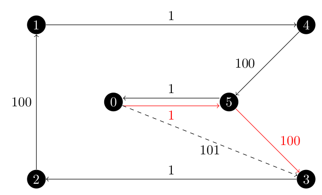
But that edge is not in the original graph, so during the post-processing done by the traveling_salesman_problem function, the red edges are inserted instead of the dashed edge.
Testing the Asadpour Algorithm#
Before I could write any tests, I needed to ensure that the tests were consistent from execution to execution.
At the time, this was not the case since there were random numbers being generated in order to sample the spanning trees.
So I had to learn how to use the @py_random_state decorator.
When this decorator is added to the top of a function, we pass it either the position of the argument in the function signature or the name of the keyword for that argument. It then takes that argument and configures a python Random object based on the input parameter.
- Parameter is
None, use a newRandomobject. - Parameter is an
int, use a newRandomobject with that seed. - Parameter is a
Randomobject, use that object as is.
So I changed the function signature of sample_spanning_tree to have random=None at the end.
For most use cases, the default value will not be changed and the results will be different every time the method is called, but if we give it an int, the same tree will be sampled every time.
But, for my tests I can give it a seed to create repeatable behaviour.
Since the sample_spanning_tree function is not visible outside of the treveling_salesman file, I also had to create a pass-through parameter for asadpour_atsp so that my seed could have any effect.
Once this was done, I modified the test for sample_spanning_tree so that it would not have a 1 in 100 chance of spontaneously failing.
At first I just passed it an int, but that forced every tree sampled to be the same (since the edges were shuffled the same and sampled from the same sequence of numbers) and the test failed.
So I tweaked it to use a Random object from the random package and this worked well.
From here, I wrap the complete asadpour_atsp parameters I want in another function fixed_asadpour like this:
def fixed_asadpour(G, weight):
    return nx_app.asadpour_atsp(G, weight, 56)


path = nx_app.traveling_salesman_problem(
    G, weight="weight", cycle=False, method=fixed_asadpour
)
I tested using both traveling_salesman_problem and asadpour_atsp.
The tests included:
- The fractional, symmetric Held Karp graph from above.
- A real world example using airline prices between six cities (also uses non-integer node names).
- The same real world example but asking for a path not a cycle.
- Using a disconnected graph (raises exception).
- Using an incomplete graph (raises exception).
- Using an integral Held Karp solution (returns directly after Held Karp with exact solution).
- Using an impossible graph (one vertex has only out edges).
Bonus Feature#
There is even a bonus feature!
The asadpour_atsp function accepts a fourth argument, source!
Since both of the return methods use eulerian_circuit and the _shortcutting functions, I can pass a source vertex to the circuit function and ensure that the returned path starts and returns to the desired vertex.
Access it by wrapping the method, just be sure that the source vertex is in the graph to avoid an exception.
def fixed_asadpour(G, weight):
    return nx_app.asadpour_atsp(G, weight, source=0)


path = nx_app.traveling_salesman_problem(
    G, weight="weight", cycle=False, method=fixed_asadpour
)References#
A. Asadpour, M. X. Goemans, A. Madry, S. O. Gharan, and A. Saberi, An O (log n / log log n)-approximation algorithm for the asymmetric traveling salesman problem, SODA ’10, Society for Industrial and Applied Mathematics, 2010, https://dl.acm.org/doi/abs/10.5555/1873601.1873633.